Modern machining combines digital and physical activities. MSC’s Dr. Tony Schmitz describes the steps that are necessary to select stable machining parameters.
Today’s machining often includes digital activities such as CAD and CAM, but the physical constraints also must be considered.
A stability map enables accurate selection of stable machining parameters.
Tool tip frequency response functions (FRFs) and cutting force model coefficients are needed to calculate the stability map.
The cutting force model coefficients are obtained from force measurements.
Modern machining is often described in the digital domain. However, there are also physical constraints that must be considered for successful machining outcomes, including vibrations caused by the machining force. These vibrations depend on the spindle speed and depth of cut, which are selected when defining a toolpath. With nonoptimal selection of these parameters, chatter can occur, which degrades surface quality, accelerates tool wear and increases scrap rates. By combining the digital planning workflow with a physics-based approach that considers the machining dynamics, manufacturers can select stable cutting parameters with confidence.
Understanding the Digital Machining Workflow
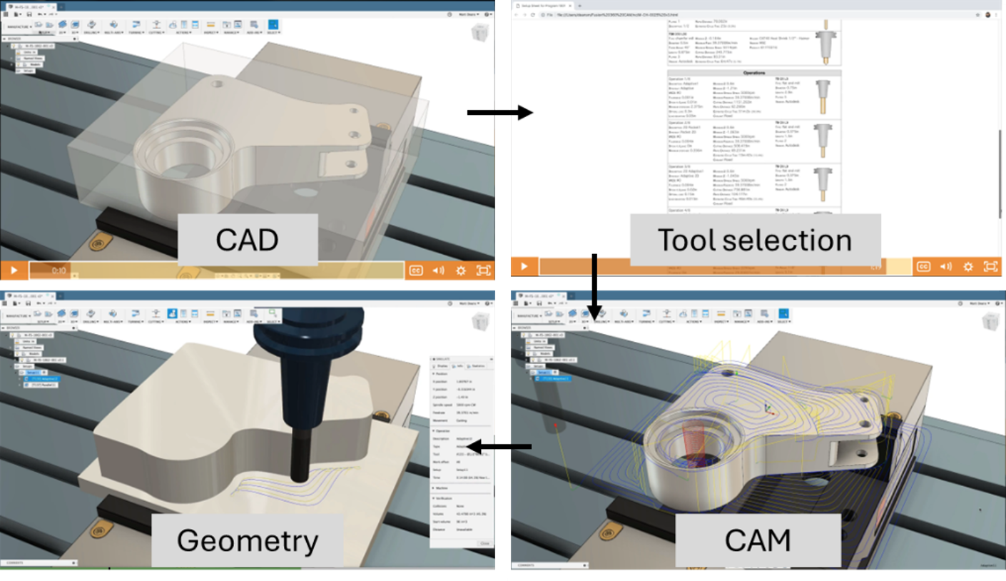
The digital machining steps are summarized in Fig. 1.
The part is designed using CAD software.
The cutting tools are selected that will be used to remove material from the preform (e.g., bar stock, forging, casting or additively manufactured preform), and the tool list is prepared with information about the toolholder geometry.
The toolpaths are generated using CAM software to produce the final design from the preform. This process is becoming increasingly automated, including support from artificial intelligence algorithms to automatically identify features and select toolpaths.
The material is removed by following the toolpaths.
Figure 1: Digital machining steps, proceeding clockwise from upper left.
Considering the Physical Constraints
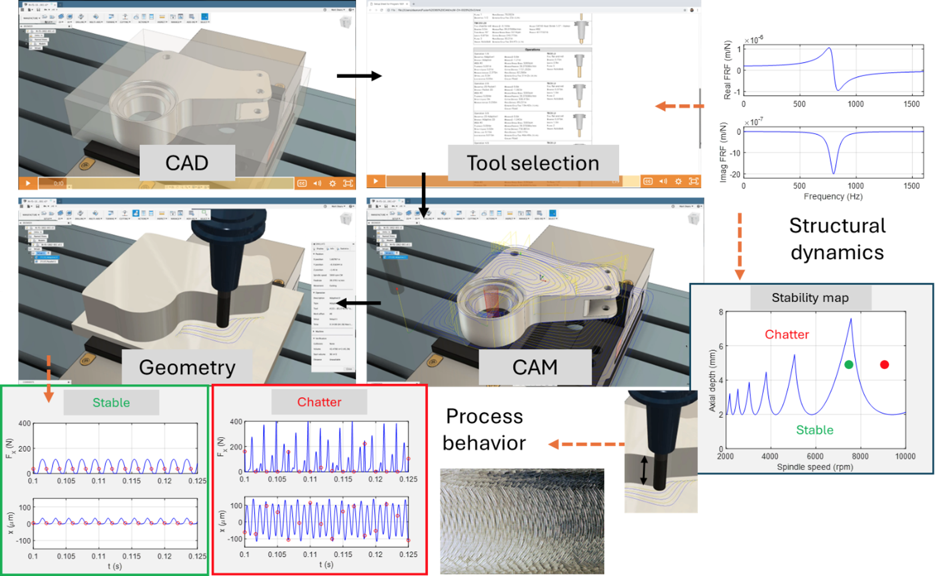
As stated, machining is more than geometry. We must also consider the physical constraints imposed by the machining dynamics. The physical machining considerations based on machining dynamics are added to the digital steps in Fig. 2.
Figure 2: Addition of the physical considerations based on machining dynamics to the digital machining steps. Compare with Fig. 1 to identify these physical considerations.
Calculating the Stability Map
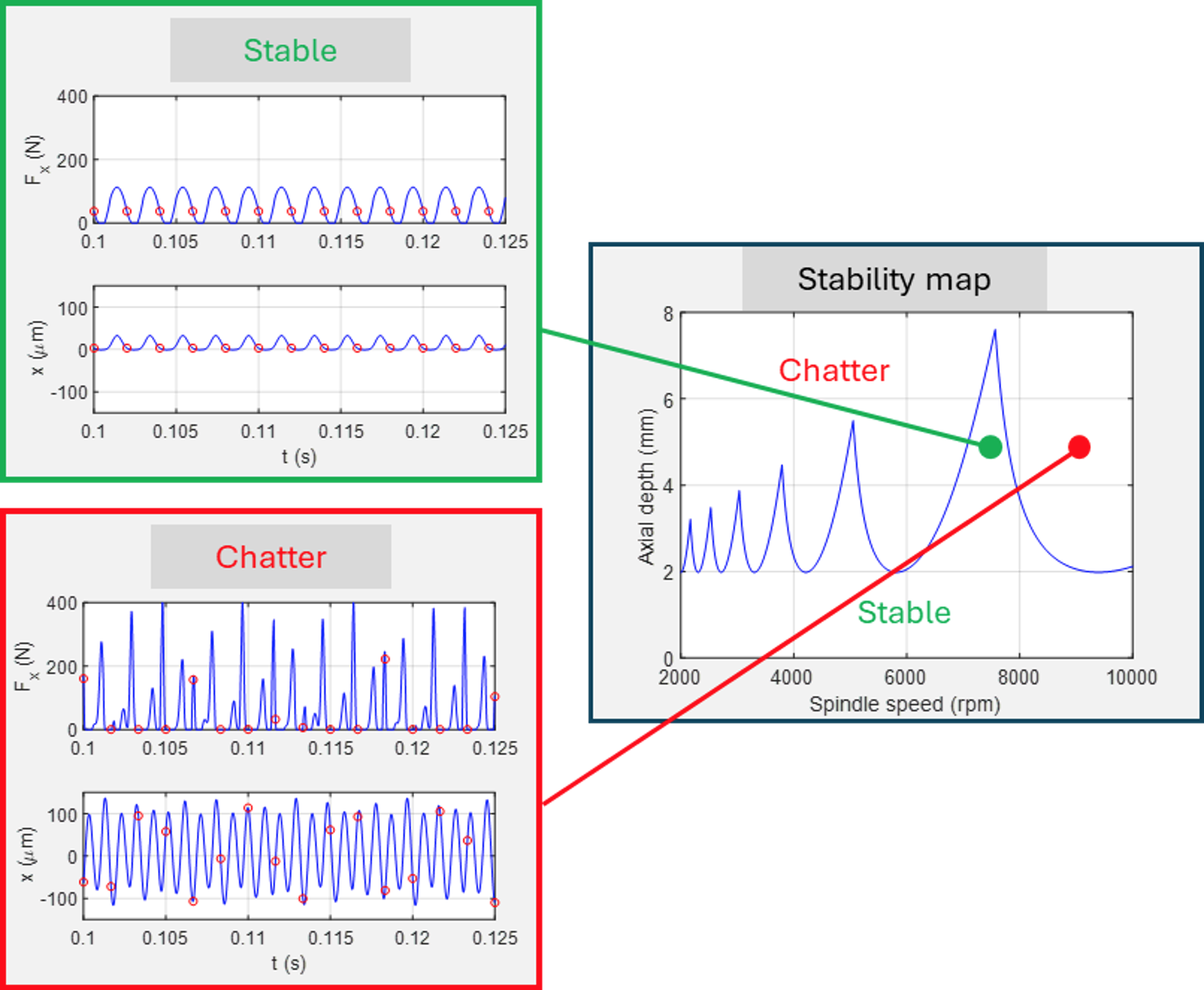
The stability map on the right-hand side of Fig. 2 separates combinations of spindle speed and axial depth that produce chatter (i.e., above the blue boundary) from those that do not (below the boundary). This enables the selection of stable machining parameters without trial and error. See Fig. 3.
Figure 3: Milling stability map.
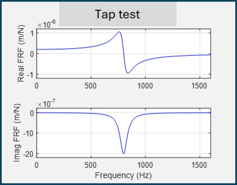
There are two primary inputs for calculating the Fig. 3 stability map using a physics-based algorithm, including time domain and frequency domain approaches. These two inputs are 1) the tool tip frequency response functions (FRFs) in the x (feed) and y directions and 2) the coefficients for a cutting force model that represents the part material and cutting tool combination. The FRFs are typically measured using the tap test; see Fig. 4 for an example result.
Figure 4: Example tap test result. The blue curve relates the input force and output displacement in the frequency domain. The minimum peak in the bottom panel identifies the natural frequency for this example.
Determining the Cutting Force Model Coefficients
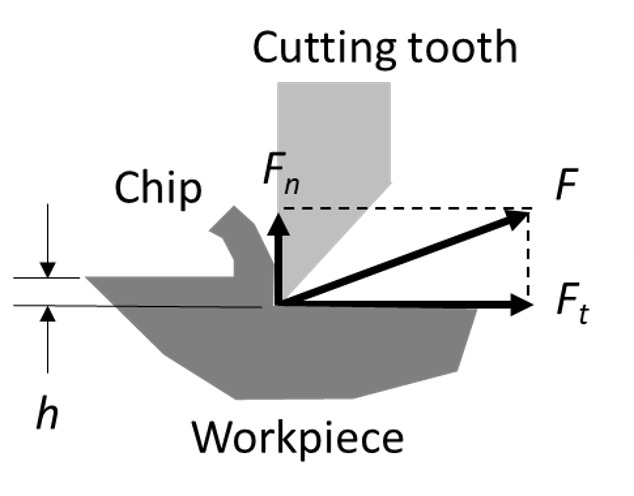
The cutting force model coefficients (k) are determined by measuring the cutting force components (F) and fitting a model. See Fig. 5 and Eqs. 1 and 2, where b is the chip width (into the page in Fig. 5), h is the chip thickness, t is the tangential force direction (i.e., the cutting speed direction) and n is the normal force direction. The cutting force model coefficients are obtained from force measurements using a cutting force dynamometer [1] or force predictions using finite element analysis (FEA) software and a material flow stress model [2].
(1) Ft = ktbh
(2) Fn = knbh
Figure 5: Cutting force components.
References
Schmitz, T. and Smith, K.S., 2019, Machining Dynamics: Frequency Response to Improved Productivity, Second Edition, Springer, New York, NY.
Dr. Tony Schmitz is a distinguished technical fellow at MSC who offers a rare blend of deep academic rigor and real-world manufacturing insight. He has a Ph.D. in mechanical engineering and more than 25 years of experience in machining dynamics, vibration, metrology and advanced manufacturing. He has authored more than 200 peer-reviewed papers as well as three engineering textbooks, and he holds 12 U.S. patents.
To request a quote, please login to your existing account or register a new one. This helps us provide you with a personalized experience and keep track of your requests.