Machine learning can model manufacturing behavior that’s difficult to capture with physics alone. MSC’s Dr. Tony Schmitz walks through a practical example showing how to get the job done.
Machine learning can predict the outcomes of a process by learning from sensor data.
Process damping is a good candidate for a machine learning approach.
Machining tests can provide training data for a stability map model that predicts stable cutting conditions.
Artificial intelligence (AI) is a topic of significant interest in manufacturing. Machine learning is a subset of AI that enables the prediction of process outcomes without explicitly being programmed. Machine learning is a data-driven modeling approach that learns from sensor data.
Using Physics-Informed Machine Learning to Include Process Damping
To demonstrate machine learning, let’s consider the application of the k-nearest neighbors (KNN) algorithm to modeling milling stability with process damping effects. Specifically, we will implement a physics-informed machine learning model to predict milling stability with process damping effects [1].
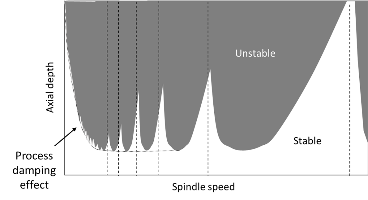
Process damping increases the stability boundary at low spindle speeds. It has been described as energy dissipation due to interference between the relief (flank) face of the cutting edge and the machined surface; see Fig. 1. Process damping is difficult to quantify using a physics-based model and, therefore, represents a good candidate for a physics-informed machine learning approach.
Figure 1: Process damping effect on the stability boundary in milling.
The KNN model is a supervised learning classifier. It uses proximity to predict the behavior at a selected data point based on the surrounding points, where the assumption is that similar points are found near one another. For milling stability classification, a class label (stable or unstable) for a new point is assigned using a majority vote from the surrounding points. The label that is most frequently represented around the new spindle speed-axial depth combination is used to predict the behavior at that point. KNN advantages are ease of implementation and low computational expense.
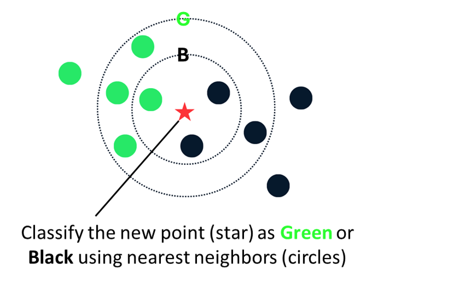
The KNN approach is described using Fig. 2. To classify (predict) the behavior at the star location, the surrounding labeled points are used. If the three nearest points (neighbors) from Fig. 2 are used, the star point will be classified as black because there are two black points and one green point among the three nearest points (i.e., the inner circle). If the seven nearest points are used, on the other hand, the star point will be classified as green because the nearest neighbors now include four green points and three black points (i.e., the outer circle).
Figure 2: KNN description.
How to Gather Data and Train the KNN Model for Machine Learning
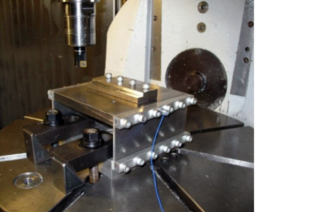
The experimental setup for the data collection and model training and validation is displayed in Fig. 3. A flexure-based setup was selected to machine an AISI 1018 steel workpiece. The up-milling conditions were 50 percent radial immersion with a 0.05 mm feed per tooth. A single-tooth indexable square endmill with a 18.54 mm diameter, 15-degree relief angle, and 0-degree rake angle was used (Kennametal model KICR073SD30333C). The flexure’s frequency response function, FRF, was measured by tap testing in the x (feed) and y directions, and the modal parameters were extracted; see Table 1 and Fig. 3. The cutting-force coefficients for the tool-work material were also identified.
Table 1: Flexure-based setup modal parameters.
Figure 3: Flexure-based milling setup.
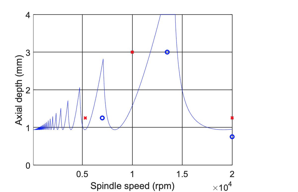
Figure 4: Stability map and initial test cut results for the setup in Fig. 3 and Table 1.
The model development begins with the physics-based stability map. As shown in Fig. 4, a map was calculated using the measured FRFs and cutting-force coefficients. Initial testing was used to validate the map. In the map, the circles represent spindle speed-axial depth combinations that were stable. The red crosses represent spindle speed-axial depth combinations that exhibited chatter. The map was used to generate a training dataset for the KNN algorithm. A grid of points was defined with 50 rpm increments in spindle speed and 250 µm increments in axial depth. Points below the stability boundary were labeled “stable,” while points above the boundary were labeled “unstable.”
Based on the training data, the Matlab fitcknn function was used to generate the KNN classifier (stability model). The KNN model used the five nearest neighbors (points), where the Euclidean distance was applied to identify the nearest neighbors. To approximately match scaling in the vertical (axial depth) and horizontal (spindle speed) axes, the axial depth was converted to units of µm. This model did not include process damping.
Testing the Model
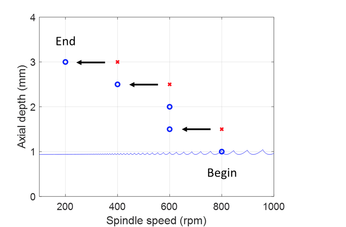
To add process damping, a stairstep approach was selected with a minimum number of cutting tests. Based on the low-flexure natural frequency (228 hertz), a spindle speed of 800 rpm was selected for the first test. A conservative axial depth of 1 mm was chosen given the predicted stability map with no process damping displayed in Fig. 4. Depending on the result of a test, a predefined progression was followed:
If the cut was stable, the spindle speed was maintained, and the axial depth was increased by 0.5 mm (50 percent of the original axial depth).
This was repeated until an unstable result was achieved at the selected spindle speed.
When an unstable cut was obtained, the spindle speed was reduced by 200 rpm (25 percent of the original spindle speed), and the previous unstable cutting depth was selected.
The sequence was repeated.
Updating the Model
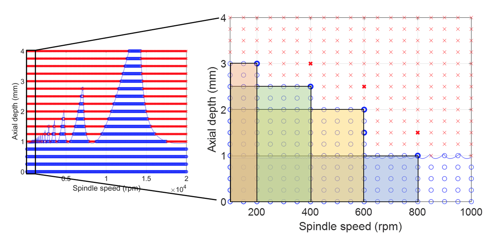
Eight test cuts were completed. The results are displayed in Fig. 5, where the original stability boundary with no process damping is shown as the blue line. Using the eight test cuts, knowledge about process damping was applied to update the full grid of initial training points. For a stable cut at a selected spindle speed-axial depth combination, all points with an equal or smaller axial depth and equal or lower spindle speed were labeled as stable. This strategy provided many updating points from a single test and is referred to here as stairstep updating. See Fig. 6 for the updating results.
Figure 5: Test results to identify process damping behavior.
Figure 6: Updating results.
Predicting Stability
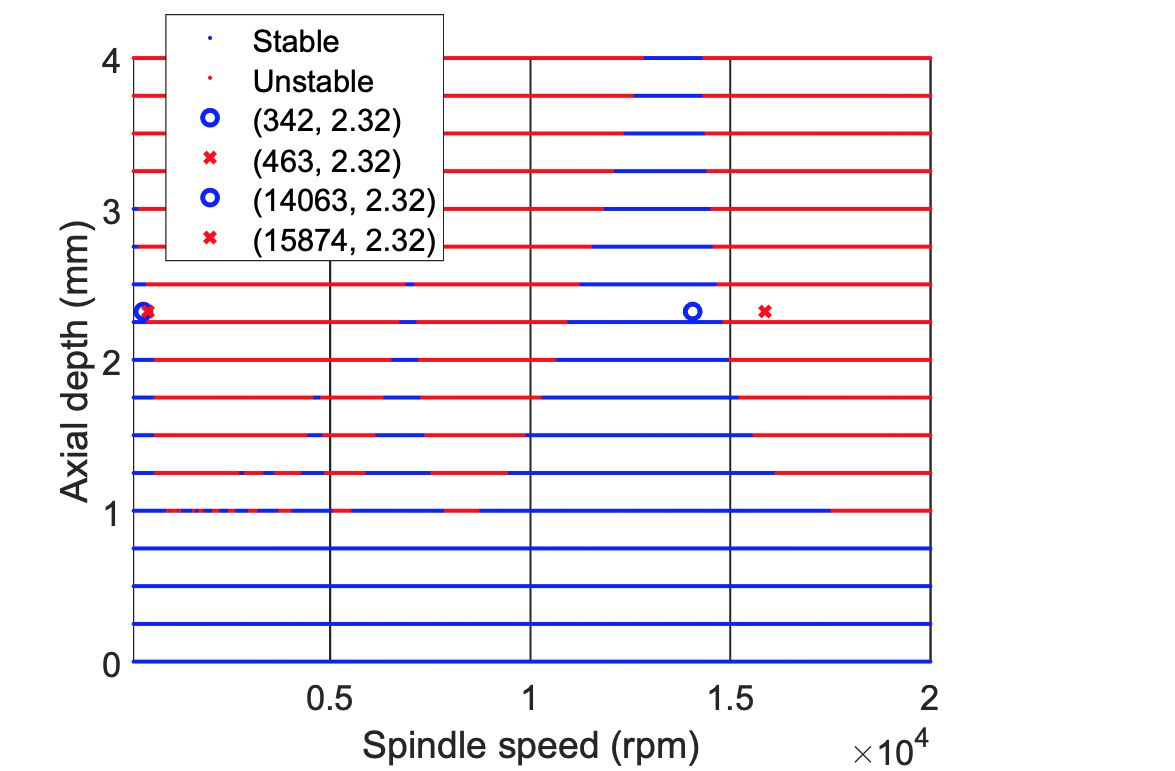
Based on the new training data in Fig. 6, the Matlab fitcknn function was again used to generate the KNN classifier with five nearest neighbors. The classifier was used to predict stability at four spindle speed-axial depth combinations not contained in the training data set. The results are provided in Fig. 7; the model successfully predicted the performance at four new points, including the effects of process damping.
Figure 7: Final KNN model with four test points for validation, including process damping effects.
References
Schmitz, T., 2024, Physics-Informed KNN Milling Stability Model with Process Damping Effects, Journal of Manufacturing Processes, 120: 1124-1129.
Dr. Tony Schmitz is a distinguished technical fellow at MSC who offers a rare blend of deep academic rigor and real-world manufacturing insight. He has a Ph.D. in mechanical engineering and more than 25 years of experience in machining dynamics, vibration, metrology and advanced manufacturing. He has authored more than 200 peer-reviewed papers as well as three engineering textbooks, and he holds 12 U.S. patents.
To request a quote, please login to your existing account or register a new one. This helps us provide you with a personalized experience and keep track of your requests.